前面博文 【opencv dnn模块 示例(3) 目标检测 object_detection (2) YOLO object detection】 介绍了 使用opencv dnn模块加载yolo weights格式模型的详细说明。 又在博文 【TensorRt(4)yolov3加载测试】 说明了如何将onnx编译为tensorrt格式并使用的方式,但是存在后处理繁琐的问题。本文将继续说明tensorrt加载yolov3模型进行推理,并且增加efficient nms trt模块。
文章目录
- 1、yolov3.weight模型格式转换
- 2、添加 EfficientNMS_TRT 层
- 2.1、添加 Reshape层
- 2.2、添加 EfficentNMS 层
- 2.3、使用 trtexec 导出优化后的模型
- 2.4、Tensorrt API c++测试 yolo_nms
- 3、c++ API实现添加NMS并推理测试
- 3.1、扩展维度
- 3.2、添加nms层
- 3.3、完整测试代码
1、yolov3.weight模型格式转换
我们先下载项目 Yolov3_Darknet_PyTorch_Onnx_Converter,配置好环境周将weights格式进行转换onnx格式,以yolov3.weights为例
python converter.py yolov3.cfg yolov3.weights 416 416
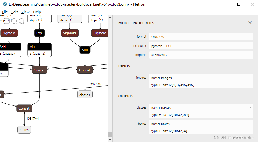
之后,会保存pt和onnx两个转换后的模型文件。通过netron查看yolov3.onnx信息,常规的三个分支输出被整合,并且仅保留80个classes 信息和 4个rect信息。
可以直接使用yolov3博文中的opencv dnn 测试代码,仅将后处理修改为如下即可
void postprocess(Mat& frame, const std::vector<Mat>& outs, Net& net)
{
    std::vector<int> classIds;
    std::vector<float> confidences;
    std::vector<Rect> boxes;

	for(int i = 0; i < outs[0].rows; i++)
	{
        Mat scores = outs[1].row(i);
        Point classIdPoint;
        double confidence;
        minMaxLoc(scores, 0, &confidence, 0, &classIdPoint);

        if(confidence > confThreshold) {
            Mat rect = outs[0].row(i);
            int centerX = (int)(rect.at<float>(0) * frame.cols);
            int centerY = (int)(rect.at<float>(1) * frame.rows);
            int width = (int)(rect.at<float>(2) * frame.cols);
            int height = (int)(rect.at<float>(3) * frame.rows);
            int left = centerX - width / 2;
            int top = centerY - height / 2;

            classIds.push_back(classIdPoint.x);
            confidences.push_back((float)confidence);
            boxes.push_back(Rect(left, top, width, height));
        }
    }

    std::vector<int> indices;
    NMSBoxes(boxes, confidences, confThreshold, nmsThreshold, indices);
    for(size_t i = 0; i < indices.size(); ++i) {
        int idx = indices[i];
        Rect box = boxes[idx];
        drawPred(classIds[idx], confidences[idx], box.x, box.y,
                 box.x + box.width, box.y + box.height, frame);
    }
}
测试结果正常
2、添加 EfficientNMS_TRT 层
在前面生成的 yolov3.onnx 模型后,通过 onnx_graphsurgeon 为其添加层类型为 EfficientNMS_TRT 的 nms处理模块。
注意: onnx模型添加EfficientNMS_TRT 仅支持 Tensorrt 作为后端推理。
首先我们需要知道EfficientNMS_TRT的输入和输出格式(更多信息点击查看),
- 输入:
- boxes : [batch_size, number_boxes, 4] or [batch_size, number_boxes, number_classes, 4]
- scores : [batch_size, number_boxes, number_classes]
- 输出:
- num_detections: [batch_size, 1], int32
- detection_boxes: [batch_size, max_output_boxes, 4]
- detection_scores: [batch_size, max_output_boxes]
- detection_classes: [batch_size, max_output_boxes], int32
2.1、添加 Reshape层
yolov3.onnx 的输出是 10647x4 和 10647x80,分别来自节点 /Concat_3 和 /Concat 而作为EfficientNMS_TRT输入仅缺少一个维度用来描述batch_size,即这里要求输入为 1x10647x4 和 1x10647x80。
我们使用 onnx_graphsurgeon 库先为onnx添加2个 Reshape节点以扩展原来两个输出的维度。
import onnx_graphsurgeon as gs
import numpy as np
import onnx

def get_nms_input(graph, class_num=1, output_name="Concat_"):
    # # input
    origin_outputs_node = [node for node in graph.nodes if node.name in output_name]

    #num_dections = origin_outputs_node[0].outputs[0].shape[0]
    #num_classes = origin_outputs_node[1].outputs[0].shape[1]

    var_classes = gs.Variable(name="classes",shape=[1] + origin_outputs_node[0].outputs[0].shape, dtype=np.float32)
    var_boxes = gs.Variable(name="boxes",shape=[1] + origin_outputs_node[1].outputs[0].shape, dtype=np.float32)

    origin_outputs_node[0].outputs[0].name = "classes_ori"  # 不能同名
    origin_outputs_node[1].outputs[0].name = "boxes_ori"

    node_classes = gs.Node(op='Reshape', name='reshape_classes',
                            inputs=[origin_outputs_node[0].outputs[0],
                                    gs.Constant('new_classes_shape', values=np.array(var_classes.shape, dtype=np.int64))],
                            outputs=[var_classes])
    node_boxes = gs.Node(op='Reshape', name='reshape_boxes',
                            inputs=[origin_outputs_node[1].outputs[0],
                                    gs.Constant('new_boxes_shape', values=np.array(var_boxes.shape, dtype=np.int64))],
                           outputs=[var_boxes])

    graph.nodes.extend([node_classes, node_boxes,])
    graph.outputs = [node_classes.outputs[0], node_boxes.outputs[0],]

    graph.cleanup().toposort()
    onnx.save(gs.export_onnx(graph),"./yolov3_extend.onnx")

	## 中间结果保存
    # graph.cleanup().toposort()
    # onnx.save(gs.export_onnx(graph),"./yolov3_extend.onnx")

    return graph

if __name__ == "__main__":
    onnx_path = "yolov3.onnx"
    graph = gs.import_onnx(onnx.load(onnx_path))

    # # 添加op得到Efficient NMS plugin的input
    graph = get_nms_input(graph,class_num=80,output_name=("/Concat_3","/Concat"))
我们运行后查看中间结果
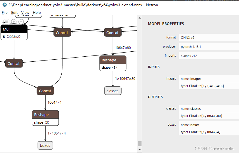
使用opencv dnn 或 使用tensorrt 导出优化编译模型均正常。
2.2、添加 EfficentNMS 层
在2.1中的代码下,添加一个函数用于在main函数中为onnx模型增加nms功能。
def create_and_add_plugin_node(graph, max_output_boxes):

    batch_size = graph.inputs[0].shape[0]
    print("The batch size is: ", batch_size)
    input_h = graph.inputs[0].shape[2]
    input_w = graph.inputs[0].shape[3]

    tensors = graph.tensors()
    boxes_tensor = tensors["boxes"]
    confs_tensor = tensors["classes"]

    num_detections = gs.Variable(name="num_detections").to_variable(dtype=np.int32, shape=[batch_size, 1])
    nmsed_boxes = gs.Variable(name="detection_boxes").to_variable(dtype=np.float32, shape=[batch_size, max_output_boxes, 4])
    nmsed_scores = gs.Variable(name="detection_scores").to_variable(dtype=np.float32, shape=[batch_size, max_output_boxes])
    nmsed_classes = gs.Variable(name="detection_classes").to_variable(dtype=np.int32, shape=[batch_size, max_output_boxes])

    new_outputs = [num_detections, nmsed_boxes, nmsed_scores, nmsed_classes]

    mns_node = gs.Node(
        op="EfficientNMS_TRT",
        attrs=create_attrs(max_output_boxes),
        inputs=[boxes_tensor, confs_tensor],
        outputs=new_outputs)

    graph.nodes.append(mns_node)
    graph.outputs = new_outputs

    return graph.cleanup().toposort()


def create_attrs(max_output_boxes=100):

    attrs = {}

    attrs["score_threshold"] = 0.25
    attrs["iou_threshold"] = 0.45
    attrs["max_output_boxes"] = max_output_boxes
    attrs["background_class"] = -1
    attrs["score_activation"] = False
    attrs["class_agnostic"] = True
    attrs["box_coding"] = 1
    # 001 is the default plugin version the parser will search for, and therefore can be omitted,
    # but we include it here for illustrative purposes.
    attrs["plugin_version"] = "1"

    return attrs


if __name__ == "__main__":
    onnx_path = "yolov3.onnx"
    graph = gs.import_onnx(onnx.load(onnx_path))

    # # 添加op得到Efficient NMS plugin的input
    graph = get_nms_input(graph,class_num=80,output_name=("/Concat_3","/Concat"))

    # # 添加Efficient NMS plugin
    graph = create_and_add_plugin_node(graph, 100)

    # # 保存图结构
    onnx.save(gs.export_onnx(graph),"yolov3_nms.onnx")
重新运行程序,查看添加后onnx网络结构如下:
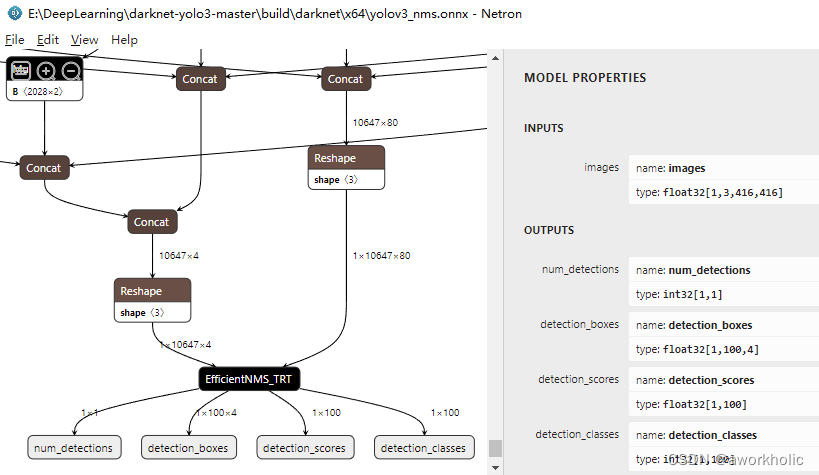
2.3、使用 trtexec 导出优化后的模型
使用命令如下:
trtexec.exe --onnx=E:\DeepLearning\darknet-yolo3-master\build\darknet\x64\yolov3_nms.onnx --saveEngine=E:\DeepLearning\darknet-yolo3-master\build\darknet\x64\yolov3_nms.onnx.engine --fp16
转换成功信息如下,可以明确看到有1个输入,4个输出。
[06/25/2024-12:25:46] [I] Using random values for input images
[06/25/2024-12:25:46] [I] Input binding for images with dimensions 1x3x416x416 is created.
[06/25/2024-12:25:46] [I] Output binding for num_detections with dimensions 1x1 is created.
[06/25/2024-12:25:46] [I] Output binding for detection_boxes with dimensions 1x100x4 is created.
[06/25/2024-12:25:46] [I] Output binding for detection_scores with dimensions 1x100 is created.
[06/25/2024-12:25:46] [I] Output binding for detection_classes with dimensions 1x100 is created.
[06/25/2024-12:25:46] [I] Starting inference
[06/25/2024-12:25:49] [I] Warmup completed 23 queries over 200 ms
[06/25/2024-12:25:49] [I] Timing trace has 347 queries over 3.01801 s
[06/25/2024-12:25:49] [I]
[06/25/2024-12:25:49] [I] === Trace details ===
[06/25/2024-12:25:49] [I] Trace averages of 10 runs:
[06/25/2024-12:25:49] [I] Average on 10 runs - GPU latency: 8.5421 ms - Host latency: 8.74631 ms (enqueue 0.733459 ms)
[06/25/2024-12:25:49] [I] Average on 10 runs - GPU latency: 8.65691 ms - Host latency: 8.86809 ms (enqueue 0.754318 ms)
[06/25/2024-12:25:49] [I] Average on 10 runs - GPU latency: 8.69078 ms - Host latency: 8.89894 ms (enqueue 0.720746 ms)
[06/25/2024-12:25:49] [I] Average on 10 runs - GPU latency: 8.53977 ms - Host latency: 8.74949 ms (enqueue 0.887427 ms)
[06/25/2024-12:25:49] [I] Average on 10 runs - GPU latency: 8.71277 ms - Host latency: 8.92263 ms (enqueue 0.95188 ms)
[06/25/2024-12:25:49] [I] Average on 10 runs - GPU latency: 8.58589 ms - Host latency: 8.79873 ms (enqueue 0.861426 ms)
[06/25/2024-12:25:49] [I] Average on 10 runs - GPU latency: 8.5209 ms - Host latency: 8.7323 ms (enqueue 0.879272 ms)
[06/25/2024-12:25:49] [I] Average on 10 runs - GPU latency: 8.62339 ms - Host latency: 8.83303 ms (enqueue 0.821729 ms)
[06/25/2024-12:25:49] [I] Average on 10 runs - GPU latency: 8.66113 ms - Host latency: 8.86626 ms (enqueue 0.718994 ms)
[06/25/2024-12:25:49] [I] Average on 10 runs - GPU latency: 8.53975 ms - Host latency: 8.74404 ms (enqueue 0.683179 ms)
[06/25/2024-12:25:49] [I]
[06/25/2024-12:25:49] [I] === Performance summary ===
[06/25/2024-12:25:49] [I] Throughput: 114.976 qps
[06/25/2024-12:25:49] [I] Latency: min = 8.62891 ms, max = 9.82397 ms, mean = 8.8045 ms, median = 8.75854 ms, percentile(90%) = 8.92554 ms, percentile(95%) = 9.17676 ms, percentile(99%) = 9.52246 ms
[06/25/2024-12:25:49] [I] Enqueue Time: min = 0.532227 ms, max = 2.55029 ms, mean = 0.750556 ms, median = 0.699585 ms, percentile(90%) = 0.886719 ms, percentile(95%) = 1.04114 ms, percentile(99%) = 1.60669 ms
[06/25/2024-12:25:49] [I] H2D Latency: min = 0.176514 ms, max = 0.218506 ms, mean = 0.190991 ms, median = 0.190277 ms, percentile(90%) = 0.199463 ms, percentile(95%) = 0.20459 ms, percentile(99%) = 0.213135 ms
[06/25/2024-12:25:49] [I] GPU Compute Time: min = 8.41919 ms, max = 9.6019 ms, mean = 8.59789 ms, median = 8.55249 ms, percentile(90%) = 8.70782 ms, percentile(95%) = 8.96716 ms, percentile(99%) = 9.30908 ms
[06/25/2024-12:25:49] [I] D2H Latency: min = 0.00976563 ms, max = 0.0393066 ms, mean = 0.0156149 ms, median = 0.015625 ms, percentile(90%) = 0.0187988 ms, percentile(95%) = 0.019165 ms, percentile(99%) = 0.0251465 ms
[06/25/2024-12:25:49] [I] Total Host Walltime: 3.01801 s
[06/25/2024-12:25:49] [I] Total GPU Compute Time: 2.98347 s
[06/25/2024-12:25:49] [W] * GPU compute time is unstable, with coefficient of variance = 1.99113%.
[06/25/2024-12:25:49] [W]   If not already in use, locking GPU clock frequency or adding --useSpinWait may improve the stability.
[06/25/2024-12:25:49] [I] Explanations of the performance metrics are printed in the verbose logs.
[06/25/2024-12:25:49] [I]
&&&& PASSED TensorRT.trtexec [TensorRT v8601] # trtexec.exe --onnx=E:\DeepLearning\darknet-yolo3-master\build\darknet\x64\yolov3_nms.onnx --saveEngine=E:\DeepLearning\darknet-yolo3-master\build\darknet\x64\yolov3_nms.onnx.engine --fp16
2.4、Tensorrt API c++测试 yolo_nms
由于EfficientNMS_TRT 层属于 tensorrt的plugins中的实现,因此在解析模型文件时,需要调用nvinfer1:initLibNvInferPlugins()函数的加载开启插件模块,前向测试代码如下:
int inference_nms()
{
    Logger logger(nvinfer1::ILogger::Severity::kVERBOSE);

    std::string trtFile = R"(E:\DeepLearning\darknet-yolo3-master\build\darknet\x64\yolov3_nms.onnx.engine)";

    std::ifstream ifs(trtFile, std::ifstream::binary);
    if(!ifs) {
        return false;
    }

    ifs.seekg(0, std::ios_base::end);
    int size = ifs.tellg();
    ifs.seekg(0, std::ios_base::beg);

    std::unique_ptr<char> pData(new char[size]);
    ifs.read(pData.get(), size);
    ifs.close();

    // engine模型
    nvinfer1:initLibNvInferPlugins(&logger, ""); // 加载插件模块

    std::shared_ptr<nvinfer1::ICudaEngine> mEngine;

    SampleUniquePtr<nvinfer1::IRuntime> runtime{nvinfer1::createInferRuntime(logger.getTRTLogger())};
    mEngine = std::shared_ptr<nvinfer1::ICudaEngine>(
        runtime->deserializeCudaEngine(pData.get(), size), InferDeleter());

    auto context = SampleUniquePtr<nvinfer1::IExecutionContext>(mEngine->createExecutionContext());

    std::vector<void*> bindings(mEngine->getNbBindings());
    for(int i = 0; i < bindings.size(); i++) {
        nvinfer1::DataType type = mEngine->getBindingDataType(i);
        nvinfer1::Dims dims = mEngine->getBindingDimensions(i);
        size_t volume = std::accumulate(dims.d, dims.d + dims.nbDims, 1, std::multiplies<size_t>());
        switch(type) {
            case nvinfer1::DataType::kINT32:
            case nvinfer1::DataType::kFLOAT: volume *= 4; break;  // 明确为类型 float
            case nvinfer1::DataType::kHALF: volume *= 2; break;
            case nvinfer1::DataType::kBOOL:
            case nvinfer1::DataType::kINT8:
            default:break;
        }
        CHECK(cudaMalloc(&bindings[i], volume));
    }

    // 输入
    cv::Mat img = cv::imread(R"(E:\DeepLearning\yolov5\data\images\bus.jpg)");
    cv::Mat blob = cv::dnn::blobFromImage(img, 1 / 255., cv::Size(inpWidth, inpHeight), {0,0,0}, true, false);

    // 推理
    CHECK(cudaMemcpy(bindings[0], static_cast<const void*>(blob.data), 1 * 3 * 416 * 416 * sizeof(float), cudaMemcpyHostToDevice));
    context->executeV2(bindings.data());
    context->executeV2(bindings.data());
    context->executeV2(bindings.data());
    context->executeV2(bindings.data());

    auto t1 = cv::getTickCount();

    CHECK(cudaMemcpy(bindings[0], static_cast<const void*>(blob.data), 1 * 3 * 416 * 416 * sizeof(float), cudaMemcpyHostToDevice));
    context->executeV2(bindings.data());
    float h_input[inpWidth * inpHeight * 3];
    int h_output_0[1];   //1
    float h_output_1[1 * 100 * 4];   //1
    float h_output_2[1 * 100];   //1
    int h_output_3[1 * 100];   //1

    cudaMemcpy(h_output_0, bindings[1], 1 * sizeof(int), cudaMemcpyDeviceToHost);
    cudaMemcpy(h_output_1, bindings[2], 1 * 100 * 4 * sizeof(float), cudaMemcpyDeviceToHost);
    cudaMemcpy(h_output_2, bindings[3], 1 * 100 * sizeof(float), cudaMemcpyDeviceToHost);
    cudaMemcpy(h_output_3, bindings[4], 1 * 100 * sizeof(int), cudaMemcpyDeviceToHost);

    auto t2 = cv::getTickCount();
    std::string label = cv::format("inference time: %.2f ms", (t2 - t1) / cv::getTickFrequency() * 1000);
    std::cout << label << std::endl;
    cv::putText(img, label, cv::Point(10, 50), cv::FONT_HERSHEY_SIMPLEX, 0.5, cv::Scalar(0, 255, 0));

    // 后处理
    float x_factor = (float)img.cols / inpWidth;
    float y_factor = (float)img.rows / inpHeight;

    int numbers = *h_output_0;
    for(int i = 0; i < numbers; i++) {

        float conf = h_output_2[i];
        if(conf < scoreThreshold)
            continue;

        int clsId = h_output_3[i];

        float x = h_output_1[i * 4];
        float y = h_output_1[i * 4 + 1];
        float w = h_output_1[i * 4 + 2];
        float h = h_output_1[i * 4 + 3];

        drawPred(clsId, conf, x * 416 * x_factor, y * 416 * y_factor, w * 416 * x_factor, h * 416 * y_factor, img);
    }
    cv::imshow("res", img);
    cv::waitKey();

    // 资源释放
    cudaFree(bindings[0]);
    cudaFree(bindings[1]);

    return 0;
}
3、c++ API实现添加NMS并推理测试
直接从yolov3.onnx模型开始,流程与上面一样,这里使用 Shuffle 来进行扩展维度,再添加EfficientNMS_TRT。由于使用c++接口,使用变复杂。
若从yolov3_extend.onnx模型开始,那么仅需要添加nms层即可(注意 输入输出层的标记)。
3.1、扩展维度
这里不解释,在某个tensor后添加一个reshape层,再将这个tensorrt的输出标记为非输出节点(已确定不再是输出),并返回节点的输出tensor。
nvinfer1::ITensor* unsqueezeTensor(SampleUniquePtr<nvinfer1::INetworkDefinition>& network, nvinfer1::ITensor* inputTensor, int axis)
{
    // 获取输入张量的维度信息
    nvinfer1::Dims dims = inputTensor->getDimensions();
    // 在指定的轴上插入一个维度
    for(int i = dims.nbDims; i > axis; --i) {
        dims.d[i] = dims.d[i - 1];
    }
    dims.d[axis] = 1;
    dims.nbDims++;

    // 重新配置张量的维度
    auto layer = network->addShuffle(*inputTensor);
    layer->setReshapeDimensions(dims);
    return layer->getOutput(0);
}
3.2、添加nms层
python中通过onnx_graphsurgeon 添加EfficientNMS_TRT 非常简单,设定参数,明确输出输出即可。c++中需要如下几个步骤:
-
- 加载插件,获取插件注册器 IPluginRegistry
-
- 通过创建器,获取指定名称( “EfficientNMS_TRT”) 插件的创建器 IPluginCreator
-
- 使用 PluginField 结构指定插件的参数数组
-
- 准备 创建器 需要的参数 PluginFieldCollection,其由 PluginField 数组构造
-
- 创建一个插件对象 IPlugin
-
- 添加插件对象到 network 中
-
- 设置添加的层的输出的名称,并标记为输出
在第三步中,PluginField 的参数类型如何设定,需要参考 对应层EfficientNMS_TRT的源代码,可以参考源代码efficientNMSPlugin.cpp 的参数说明和创建代码
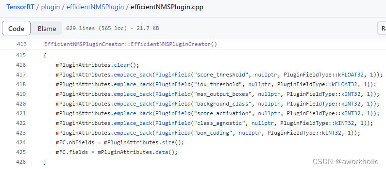
本文中添加插件层的代码实现,如下
    // 1
	nvinfer1:initLibNvInferPlugins(&logger, "");
    auto registry = nvinfer1::getBuilderPluginRegistry(nvinfer1::EngineCapability::kDEFAULT);
    // 2
    auto creator = registry->getPluginCreator("EfficientNMS_TRT", "1");
	// 3
    auto score_threshold = 0.25f;
    auto iou_threshold = 0.45f;
    auto max_output_boxes = 100;
    auto background_class = -1;
    auto score_activation = 0;
    auto class_agnostic = 1;
    auto box_coding = 1;
    //auto plugin_version = "1";
    std::vector<nvinfer1::PluginField> new_pluginData_list = {
        {"score_threshold", &score_threshold, PluginFieldType::kFLOAT32, sizeof(score_threshold)},
        {"iou_threshold", &iou_threshold, PluginFieldType::kFLOAT32, sizeof(iou_threshold)},
        {"max_output_boxes", &max_output_boxes, PluginFieldType::kINT32, sizeof(max_output_boxes)},
        {"background_class", &background_class, PluginFieldType::kINT32, sizeof(background_class)},
        {"score_activation", &score_activation, PluginFieldType::kINT32, sizeof(score_activation)},
        {"class_agnostic", &class_agnostic, PluginFieldType::kINT32, sizeof(class_agnostic)},
        {"box_coding", &box_coding, PluginFieldType::kINT32, sizeof(box_coding)},
        //{"plugin_version", &plugin_version, PluginFieldType::kCHAR, sizeof(plugin_version)},
    };
	// 4
    auto collection = nvinfer1::PluginFieldCollection();
    collection.nbFields = new_pluginData_list.size();
    collection.fields = new_pluginData_list.data();
	// 5
    auto plugin = creator->createPlugin("nms_layer", &collection);
	// 6
    auto layer = network->addPluginV2(newOutputsTensors.data(), newOutputsTensors.size(), *plugin);
    layer->getOutput(0)->setName("det_num");
    layer->getOutput(1)->setName("det_boxes");
    layer->getOutput(2)->setName("det_scores");
    layer->getOutput(3)->setName("det_classes");
    // 7
    network->markOutput(*layer->getOutput(0));
    network->markOutput(*layer->getOutput(1));
    network->markOutput(*layer->getOutput(2));
    network->markOutput(*layer->getOutput(3));
3.3、完整测试代码
测试代码如下,正常。
void build()
{
    std::string onnxFile = R"(E:\DeepLearning\darknet-yolo3-master\build\darknet\x64\yolov3.onnx)";

    Logger logger(nvinfer1::ILogger::Severity::kVERBOSE);

    /// 1.2 优化需要使用的临时变量
    // builder
    auto builder = SampleUniquePtr<nvinfer1::IBuilder>(nvinfer1::createInferBuilder(logger));

    // network
    const auto explicitBatch = 1U << static_cast<uint32_t>(nvinfer1::NetworkDefinitionCreationFlag::kEXPLICIT_BATCH);
    auto network = SampleUniquePtr<nvinfer1::INetworkDefinition>(builder->createNetworkV2(explicitBatch));

    // onnx parser
    auto parser = SampleUniquePtr<nvonnxparser::IParser>(nvonnxparser::createParser(*network, logger));
    auto parsed = parser->parseFromFile(onnxFile.c_str(), (int)nvinfer1::ILogger::Severity::kVERBOSE);

    //  extend dims
    //  scores [10647,80] -> [1, 10647,80],  boxex[10647,4] -> [1, 10647,4],
    int nbOut = network->getNbOutputs(); // 2
    std::vector<nvinfer1::ITensor*> outputsTensors(2);
    outputsTensors[0] =  network->getOutput(1);
    outputsTensors[1] = network->getOutput(0);
    for(auto tensor : outputsTensors) {
        //auto dims = tensor->getDimensions();
        //auto name = tensor->getName();
        network->unmarkOutput(*tensor);
    }

    std::vector<nvinfer1::ITensor*> newOutputsTensors = {
        unsqueezeTensor(network, outputsTensors[0], 0),
        unsqueezeTensor(network, outputsTensors[1], 0)
    };
    //for(auto tensor : newOutputsTensors) {
    //    auto dims = tensor->getDimensions();
    //    auto name = tensor->getName();
    //}

    // nms
    nvinfer1:initLibNvInferPlugins(&logger, "");

    auto registry = nvinfer1::getBuilderPluginRegistry(nvinfer1::EngineCapability::kDEFAULT);
    auto creator = registry->getPluginCreator("EfficientNMS_TRT", "1");

    auto score_threshold = 0.25f;
    auto iou_threshold = 0.45f;
    auto max_output_boxes = 100;
    auto background_class = -1;
    auto score_activation = 0;
    auto class_agnostic = 1;
    auto box_coding = 1;
    auto plugin_version = "1";
    std::vector<nvinfer1::PluginField> new_pluginData_list = {
        {"score_threshold", &score_threshold, PluginFieldType::kFLOAT32, sizeof(score_threshold)},
        {"iou_threshold", &iou_threshold, PluginFieldType::kFLOAT32, sizeof(iou_threshold)},
        {"max_output_boxes", &max_output_boxes, PluginFieldType::kINT32, sizeof(max_output_boxes)},
        {"background_class", &background_class, PluginFieldType::kINT32, sizeof(background_class)},
        {"score_activation", &score_activation, PluginFieldType::kINT32, sizeof(score_activation)},
        {"class_agnostic", &class_agnostic, PluginFieldType::kINT32, sizeof(class_agnostic)},
        {"box_coding", &box_coding, PluginFieldType::kINT32, sizeof(box_coding)},
        //{"plugin_version", &plugin_version, PluginFieldType::kCHAR, sizeof(plugin_version)},
    };

	auto collection = nvinfer1::PluginFieldCollection();
    collection.nbFields = new_pluginData_list.size();
    collection.fields = new_pluginData_list.data();

    auto plugin = creator->createPlugin("nms_layer", &collection);

    auto layer = network->addPluginV2(newOutputsTensors.data(), newOutputsTensors.size(), *plugin);
    layer->getOutput(0)->setName("det_num");
    layer->getOutput(1)->setName("det_boxes");
    layer->getOutput(2)->setName("det_scores");
    layer->getOutput(3)->setName("det_classes");
    network->markOutput(*layer->getOutput(0));
    network->markOutput(*layer->getOutput(1));
    network->markOutput(*layer->getOutput(2));
    network->markOutput(*layer->getOutput(3));

    // config
    auto config = SampleUniquePtr<nvinfer1::IBuilderConfig>(builder->createBuilderConfig());
    config->setFlag(nvinfer1::BuilderFlag::kFP16);

    auto profileStream = makeCudaStream();
    config->setProfileStream(*profileStream);

    /// 1.3 编译优化engine并序列化
// serialize
    SampleUniquePtr<nvinfer1::IHostMemory> plan{builder->buildSerializedNetwork(*network, *config)};

    std::ofstream ofs(R"(E:\DeepLearning\darknet-yolo3-master\build\darknet\x64\yolov3.onnx.nms.trt)", std::ostream::binary);
    ofs.write(static_cast<const char*>(plan->data()), plan->size());
    ofs.close();
}
![[论文笔记]Mixture-of-Agents Enhances Large Language Model Capabilities](https://img-blog.csdnimg.cn/img_convert/5d22cbef89dc60bc63c94dfa38cbf438.png)